2.0 Overview
The fundamental theoretical framework and methodology for the Genuine Progress Indicator was put forth by Herman Daly and John Cobb in their seminal book, For the Common Good, published in 1989. Daly and Cobb advocated for modifying a country’s gross domestic product (GDP) by including the costs and benefits of social and environmental factors, terming their new indicator the Index of Sustainable Economic Welfare (ISEW). In 1994 the public policy think tank Redefining Progress took the fundamentals of the ISEW and developed the Genuine Progress, making some minor methodological improvements, but keeping the fundamental approach of triple bottom line accounting.
Since inception the GPI has been calculated for many different
countries, states, and cities all around the world by a diverse group of
academic researchers, government entities, and non-profits. The
individual studies largely adhere to the formula initially conceived,
but many have made changes to the calculations that make comparison
between studies difficult. These changes were made with the best
intentions, to improve the theoretical or methodological basis of the
calculation, but the problem of incomparable results remains. A group of
GPI researchers and practitioners was convened in order to address how
the GPI could be updated to take advantage of newly available data
sources and best reflect the most current scientific understanding of
well-being. This resulted in two GPI Summits being held in Maryland in
the summer of 2012 and 2013 and an online working group, with the goal
of developing “GPI 2.0”.
This work was done in collaboration with John Talberth and Michael Weisdorf of the Center for a Sustainable Economy (sustainable-economy.org). Their report on the GPI for Baltimore in 2012 and 2013 can be found at sustainable-economy.org/genuine-progress/
GPI 2.0 Improvements
GPI 2.0 takes advantage of the increasing availability of data and the most recent scientific understanding of factors influencing our well-being. As an example of the increasing resolution of data available, the amount of money people spend on items in their daily lives was inferred from national data and considered together in GPI 1.0, whereas in 2.0 we were able to consider data gathered for household spending in Maryland broken into 17 categories. This helps us make the determination of what expenditures are contributing to well-being at a finer scale. Recent scientific literature has helped us improve the determination of several indicators, including the cost of inequality, value of ecosystem services, the cost of air pollution, and the cost of noise pollution. We are using spatial data to calculate some indicators, like the extent of forest in Maryland and the cost of air pollution.
The drawback to relying on recently available data is that it often does not extend very far into the past. For this reason, we are only able to present 2012, 2013, and 2014 calculated using the GPI 2.0 methodology. However, we will maintain the GPI 1.0 results on this website, which extends from 1960 to 2013.
Highlights from 2018-2019 GPI Update
The GPI increased by $7 billion (4%) from 2018 to 2019. The increase in the GPI was driven by increases in household budget expenditures ($3.6 billion), and a decline in the costs of income inequality ($4 billion) and underemployment ($0.79 billion) from the prior year. We did see increases in the loss of natural lands (%0.15 billion, a 10% increase) and depletion of nonrenewable energy resources ($0.29 billion, a 7% increase). Interestingly, in this case Maryland GSP aligns well with the GPI as it also increased by nearly 4% from 2018 to 2019.
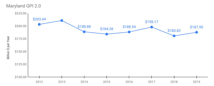
Maryland GPI
GPI Per Capita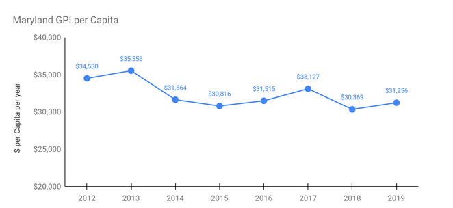
There was a $8.48 billion increase - or 3.66% - in the GPI measure
from 2014 to 2015. Improvements were seen in indicators such as
employment ($0.91 billion), external benefits from higher education
($1.28 billion), household budget expenditures ($6.74 billion), and the
value of unpaid labor (~$5 billion). Positive effects from these
benefits were somewhat dampened by increases in income inequality ($1.27
billion), costs of medical care ($0.72 billion), and the cost of crime
($2.4 billion). The significant increase in crime was primarily due to
an additional 244 murders - or a 79% increase - from 2014 to 2015. This
factor alone was the cause of a $2.2 billion increase in cost between
the two years.
Some other indicators that went through positive changes from 2014 to
2015 include services from household capital, which increased by 1.6%
($0.58 billion), internet services, which increased by 3.67% ($0.12
billion), cost of commuting (decreased by $0.30 billion, 1.73%), and
public transit, which increased by 10.72% ($0.14 billion).
From 2014 to 2015 there was a very slight increase in environmental
costs. Water pollution, solid waste, and greenhouse gas emissions
increased by 3.91%, 3.56%, and 3.09% respectively. Noise pollution
essentially held steady, and criteria air pollutants decreased by 0.39%.
As stated in the 2014 GPI update, the cost of water pollution is
calculated as expenditures associated with meeting clean water goals
(i.e. the Bay TMDL), so while spending is increasing now a clean bay
will confer benefits in the future.
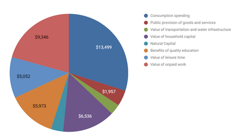 Maryland GPI Benefits Per Capita 2019
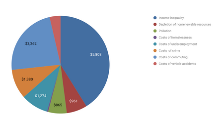 Maryland GPI Costs Per Capita 2019
Comparison of GPI 2.0 and 1.0 Results
Results are similar in trend using both 1.0 and 2.0 methods, but 2.0 shows a slightly smaller increase year over year from 2012 to 2013 (2.40% vs. 2.70%). The ending GPI value using 2.0 methods is $11 billion more than GPI 1.0 due to the fact that GPI 2.0 includes additional positive inputs, such as ecosystem services, public provisioning government spending, and services from libraries and the internet. These outweigh the additional costs considered in 2.0 like homelessness, groundwater depletion, and additional air pollutants.
